An improved multiscale finite element method for simulating two-dimensional water flow in porous media
A porous medium and finite element technology, applied in the field of hydraulics, can solve problems such as unsteady flow, achieve the effect of reducing the amount of calculation and calculation time, and high efficiency
- Summary
- Abstract
- Description
- Claims
- Application Information
AI Technical Summary
Problems solved by technology
Method used
Image
Examples
Embodiment 1
[0034] Embodiment 1: the continuum model of two-dimensional steady flow
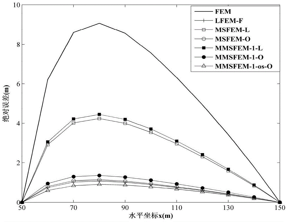
[0035] The research area is a square unit: Ω=[50m, 150m]×[50m, 150m], permeability coefficient K(x,y)=x 2 m / d. The water flow equation is formula (1), and the boundary condition is constant head boundary condition This model has an analytical solution: H=3x 2 +y 2 .
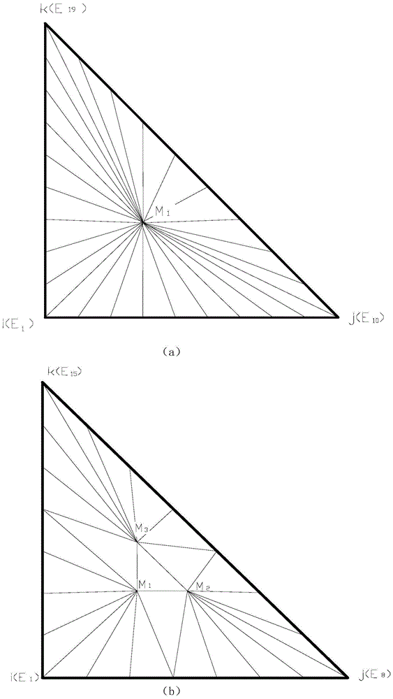
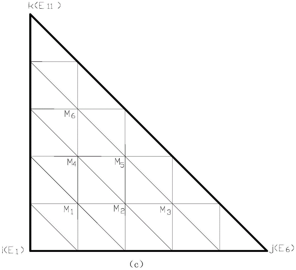
[0036] The model is solved by LFEM, LFEM-F, MSFEM-L, MSFEM-O, MMSFEM-1-L, MMSFEM-1-O, MMSFEM-1-os-O. Among them, LFEM-F divides the study area into 1800 parts, and other methods divide the study area into 200 coarse grid units. MSFEM uses the traditional triangulation method to subdivide each coarse grid into 9 units, and MMSFEM adopts the improved fine subdivision method to subdivide each coarse grid into 9 units. The super sample unit used by the super sample technology is 1.01 times of the coarse grid unit.
[0037] figure 2 For the head calculated by the above method, the absolute error of the profile at y=100m. from figure 2...
Embodiment 2
[0038] Example 2: Gradient medium model of two-dimensional unsteady flow (pumping model of flood plain)
[0039] The research area is a square unit: Ω=[0,10km]×[0m,10km], the permeability coefficient increases from 1m / d to 250m / d from the left side to the right side of the boundary of the research area, namely K(x,y)= 1+x / 40m / d. The water flow equation is formula (2), the left and right boundaries define the water head boundary, the left boundary is 10m, the right boundary is 0m, and the upper and lower water barrier boundaries. The thickness of the aquifer is 10m, and the water storage coefficient S=0.00001-0.000009x / 1000 / m. There is a pumping well at coordinates (5200m, 5200m) with a flow rate of 1000m 3 / d, the pumping time is 5 days, and the time step is 1 day. The water head H at the initial moment 0 (x, y) = 10-x / 1000m. There is no analytical solution for this model, therefore, the solution of LFEM-F is used as the standard reference.
[0040] The model is solved b...
Embodiment 3
[0041] Example 3: Two-dimensional unsteady flow abrupt change medium model
[0042] The research area is a square unit: Ω=[0,10km]×[0m,10km], the permeability coefficient changes abruptly at x=2480m, that is, when x3 / d, the pumping time is 3 days, and the time step is 1 day. The thickness of the aquifer is 10m, the water storage coefficient x0 (x, y) = 10-x / 1000m. There is no analytical solution for this model, therefore, the solution of LFEM-F is used as the standard reference.
[0043] Use LFEM, LFEM-F, MSFEM-O, MMSFEM-3-O to solve this model. Among them, LFEM-F divides the study area into 80,000 triangular units, and other methods divide the study area into 400 units. In this model, MMSFEM adopts radial subdivision, and MSFEM adopts traditional subdivision to subdivide the coarse grid unit into 100 triangular units. Figure 4 is the water head of each method y=5000m section. The accuracy of MMSFEM is very close to that of MSFEM. In this model, the CPU time required by...
PUM
 Abstract
Description
Claims
Application Information
 - R&D
- Intellectual Property
- Life Sciences
- Materials
- Tech Scout
- Unparalleled Data Quality
- Higher Quality Content
- 60% Fewer Hallucinations
Browse by: Latest US Patents, China's latest patents, Technical Efficacy Thesaurus, Application Domain, Technology Topic, Popular Technical Reports.
© 2025 PatSnap. All rights reserved.Legal|Privacy policy|Modern Slavery Act Transparency Statement|Sitemap|About US| Contact US: help@patsnap.com


