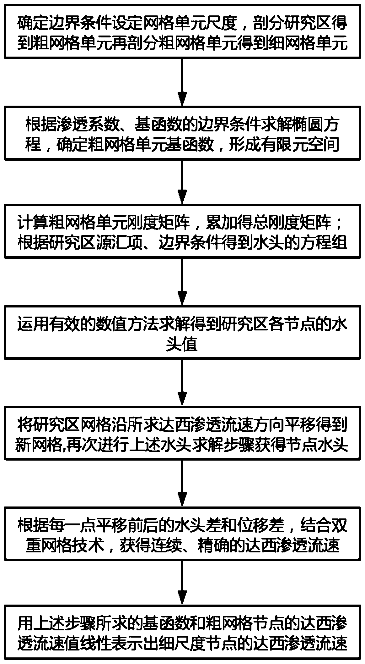
Double-grid multi-scale finite element method for simulating node Darcy permeation flow velocity
A technology for simulating nodes and finite elements, applied in the field of hydraulics, it can solve problems such as large computational consumption and low computational efficiency, and achieve the effects of high efficiency, high computational efficiency and high precision
- Summary
- Abstract
- Description
- Claims
- Application Information
AI Technical Summary
Problems solved by technology
Method used
Image
Examples
Embodiment 1
[0048] Embodiment 1: two-dimensional homogeneous medium steady flow model
[0049] The research area Ω is [0, 1]×[0, 1], the aquifer thickness is 1, the permeability coefficient K=1, the analytical solution is H=xy(1-x)(1-y), the source-sink term W and The Dirichlet boundary condition is given by the analytical solution, and the two-dimensional steady flow equation for groundwater can be expressed as:
[0050]
[0051] Coarse-scale Darcy percolation velocity
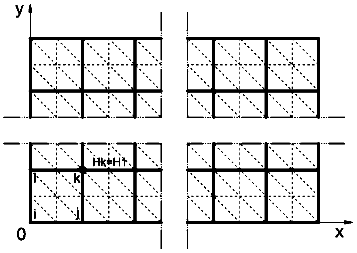
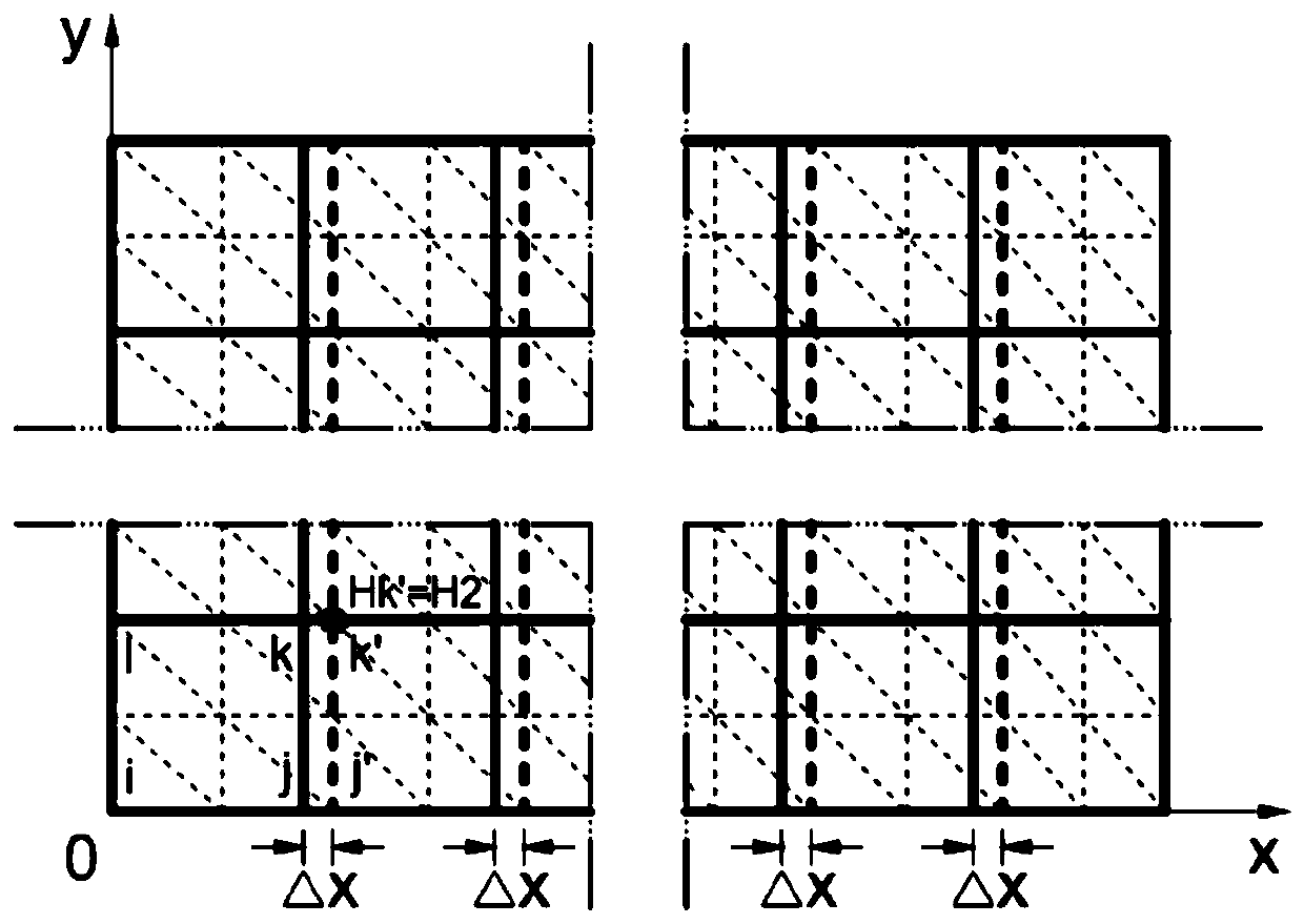
[0052] In this example, the D-MSFEM, D-FEM and Yeh methods all divide the study area into N×N parts. When N=10, 20, 30 and 40, the coarse grid unit scales are 0.1, 0.05, 0.03, 0.025. When calculating with D-FEM and Yeh method, the study area is divided into 200, 800, 1800, 3200 triangular coarse mesh units (N×N×2) corresponding to them, and when calculating with D-MSFEM method, the The study area was divided into 100, 400, 900, and 1600 square coarse grid units (N×N), and each coarse grid unit was divided into 8 tr...
Embodiment 2
[0062] Example 2: Two-dimensional high oscillating head steady flow model
[0063] The two-dimensional steady flow equation for the oscillation of the permeability coefficient is (2), and the permeability coefficient The research area Ω is [0, 1]×[0, 1], the aquifer thickness is 1, the analytical solution is H=xy(1-x)(1-y), the source-sink term W and the Dirichlet boundary condition are given by The analytical solution is given. Let the amplitude A=1.99, phase Q=1.5, then the maximum value of the permeability coefficient is 400 times of the minimum value, Figure 7 This is a schematic diagram of the three-dimensional distribution of the permeability coefficient in a heterogeneous medium.
[0064] This example is solved by Yeh-F, D-MSFEM-O, D-MSFEM-L, Yeh and D-FEM methods. The coarse grid scale was set at 0.025, and D-FEM and Yeh divided the study area into 3200 triangular coarse grid units (N×N×2). D-MSFEM divides the study area into 1600 square coarse grid units (N×N), ...
Embodiment 3
[0067] Example 3: Two-dimensional gradient medium unsteady flow model
[0068] The general equation for an unsteady flow is represented by a parabolic equation in two-dimensional form:
[0069]
[0070] In the formula, K is the permeability coefficient, H is the water head, W is the source-sink item, S is the water storage coefficient, and Ω is the study area.
[0071] The study area is [0, 10km] × [0, 10km], the boundary conditions are the upper and lower water barrier boundaries, the left and right boundaries are the first type, the left boundary water head is 10m, the right boundary water head is 0m, and the source-sink item is 0. The permeability coefficient increases slowly from left to right, specifically m / day is a typical variation characteristic of the piedmont alluvial plain medium. The time step is 1day and the total time is 5day. Since there is no analytical solution for this example, the study area is finely divided into 200×200 parts by Yeh-F, and 80,000 t...
PUM
 Abstract
Description
Claims
Application Information
 - R&D
- Intellectual Property
- Life Sciences
- Materials
- Tech Scout
- Unparalleled Data Quality
- Higher Quality Content
- 60% Fewer Hallucinations
Browse by: Latest US Patents, China's latest patents, Technical Efficacy Thesaurus, Application Domain, Technology Topic, Popular Technical Reports.
© 2025 PatSnap. All rights reserved.Legal|Privacy policy|Modern Slavery Act Transparency Statement|Sitemap|About US| Contact US: help@patsnap.com


