Heterogeneous fleet fault tolerance control method based on variable time interval strategy
A time interval, fault-tolerant control technology, applied in non-electric variable control, two-dimensional position/navigation control, vehicle position/route/altitude control, etc. Queue stability and other issues to achieve the effect of increasing critical traffic capacity and ensuring stability
- Summary
- Abstract
- Description
- Claims
- Application Information
AI Technical Summary
Problems solved by technology
Method used
Image
Examples
Embodiment 1
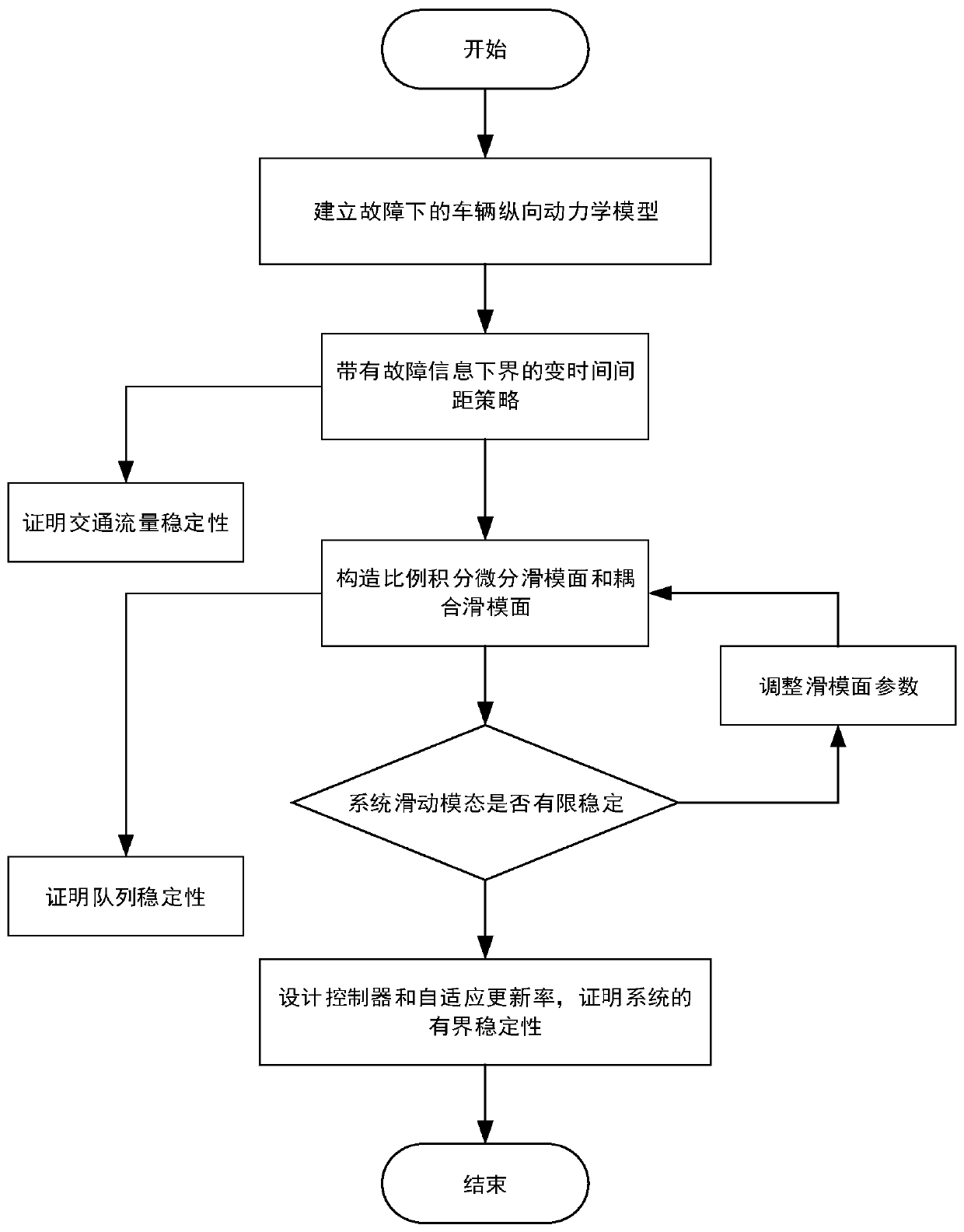
[0115] The specific process of step S1 is as follows:
[0116] S11. Define the dynamic model of the leading vehicle, as follows:
[0117]
[0118] where x0 (t), v 0 (t), a 0 (t) represent the position, speed and acceleration of the leading car respectively, and a 0 (t) represents the same given time function;
[0119] S12. Perform force analysis on the longitudinal motion of the vehicle to obtain the longitudinal dynamic model of the vehicle:
[0120]
[0121]
[0122]
[0123] where x i ,v i ,a i are the position, velocity and acceleration of vehicle i respectively; c i is the actuator input, f i (v i ,a i ) is a nonlinear function, and its function expression is as follows:
[0124]
[0125] Among them, τ i is the engine time constant, υ is the air mass constant, m i , A i , C di and d mi are the mass, cross-sectional area, drag coefficient and mechanical drag of vehicle i respectively; due to the mass m of the car i is uncertain, so the nonli...
Embodiment 2
[0136] On the basis of embodiment 1, the specific process of step S2 is as follows:
[0137] S21. Define the displacement tracking error as follows:
[0138]
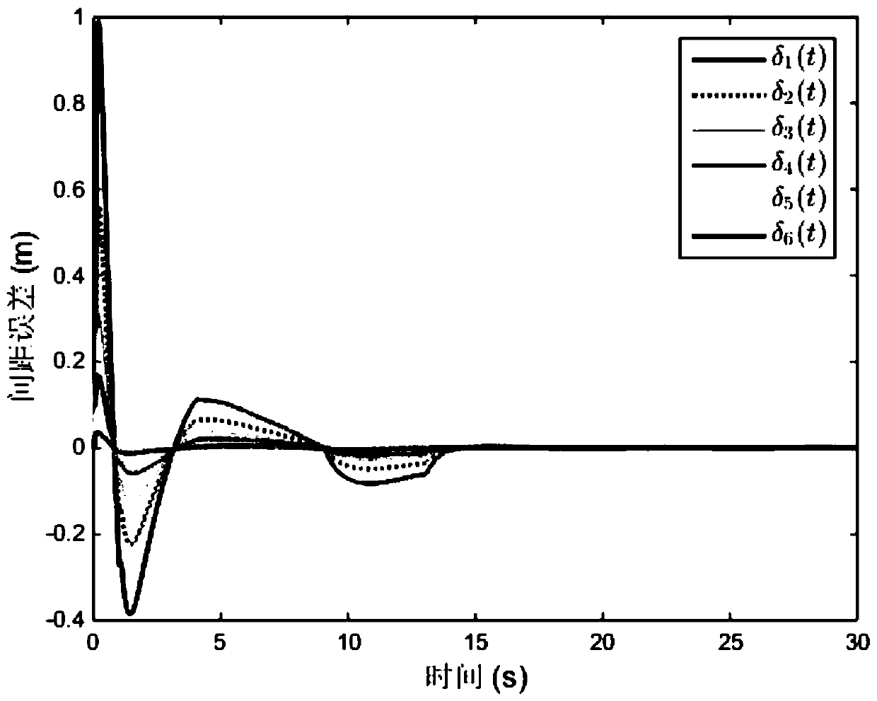
[0139] Among them, δ i is the safety distance error between the i-th car and the i-1th car, γ i is a constant, L i is the length of vehicle i, Δ i-1,i is the safety distance between two vehicles, h represents the delay time of the fleet control system, σ represents the safety factor, A m is the expected maximum acceleration of the controlled vehicle, ρ i0 Represents the lower bound value of the actuator failure; thus it can be obtained that:
[0140]
[0141] Indicates that the initial value of the proposed variable time spacing strategy is zero in any case;
[0142] S22. Define the ideal inter-vehicle distance as follows:
[0143]
Embodiment 3
[0145] On the basis of embodiment 2, the specific process of step S3 is as follows:
[0146] S31. In order to make δ i It tends to be infinitely close to 0 in a finite time and guarantees the consistent stability of the queue, constructing a proportional-integral-differential sliding surface:
[0147]
[0148] Among them, K p , K i , K d represent proportional, integral and differential coefficients respectively;
[0149] S32. According to the transfer function G i (s) definition, construct δ i and δ i+1 The relationship between , defines the coupled sliding mode surface:
[0150]
[0151] where λ is the coupled sliding mode surface s i and s i+1 normal number of ; when s i When reaching the sliding surface, s i can also reach the sliding surface.
PUM
| Property | Measurement | Unit |
|---|---|---|
| Cross-sectional area | aaaaa | aaaaa |
Abstract
Description
Claims
Application Information
 - R&D
- Intellectual Property
- Life Sciences
- Materials
- Tech Scout
- Unparalleled Data Quality
- Higher Quality Content
- 60% Fewer Hallucinations
Browse by: Latest US Patents, China's latest patents, Technical Efficacy Thesaurus, Application Domain, Technology Topic, Popular Technical Reports.
© 2025 PatSnap. All rights reserved.Legal|Privacy policy|Modern Slavery Act Transparency Statement|Sitemap|About US| Contact US: help@patsnap.com


