Systems and methods for construction of time-frequency surfaces and detection of signals
a time-frequency surface and detection system technology, applied in the field of signal processing, can solve the problems of high sampling rate, inability to address, and delay in real-time processing
- Summary
- Abstract
- Description
- Claims
- Application Information
AI Technical Summary
Benefits of technology
Problems solved by technology
Method used
Image
Examples
example 1
Simulated Data Sources with Constant Sampling Grid
[0054]A constant sampling test was carried out with simulated input signal data that contained three simultaneous data signal sources. In the simulation, 131,072 samples were collected at 100 MHz with a bit depth of 3 bits. The first source was a 0 dB CW tone with a frequency of 38 MHz. The second source was a 0 dB CW tone with a frequency of 25.5 MHz. The third source was a 0 dB FM chirp with a frequency that swept from 11 and 16 MHz. The signals were all inserted into a background of white Gaussian noise with signal to noise ratio (SNR) of 0 dB. In the analysis, short-time Fourier Transforms were applied to the data to generate time-frequency surfaces (spectrograms), depicted in FIGS. 6a, 7a, and 8a. FIG. 6A depicts a spectrogram for the constantly sampled full set of simulated data, with 100 frequency bins equally spaced 0 to the Nyquist frequency of 50 MHz. In the spectrogram of FIG. 6A, the three data sources are clear and indic...
example 2
Randomly Sub-Sampled Data Using Streaming Time-Frequency (TF) Methodology
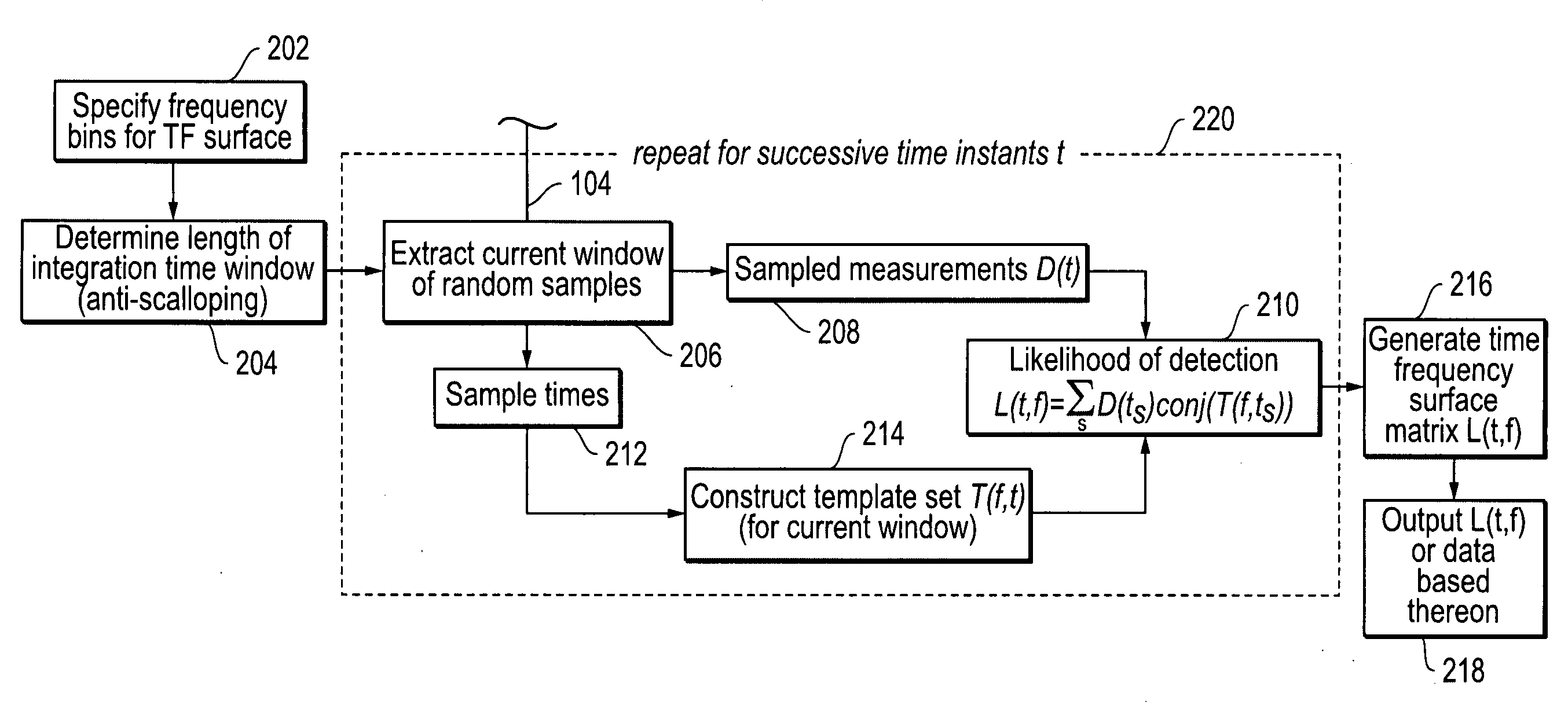
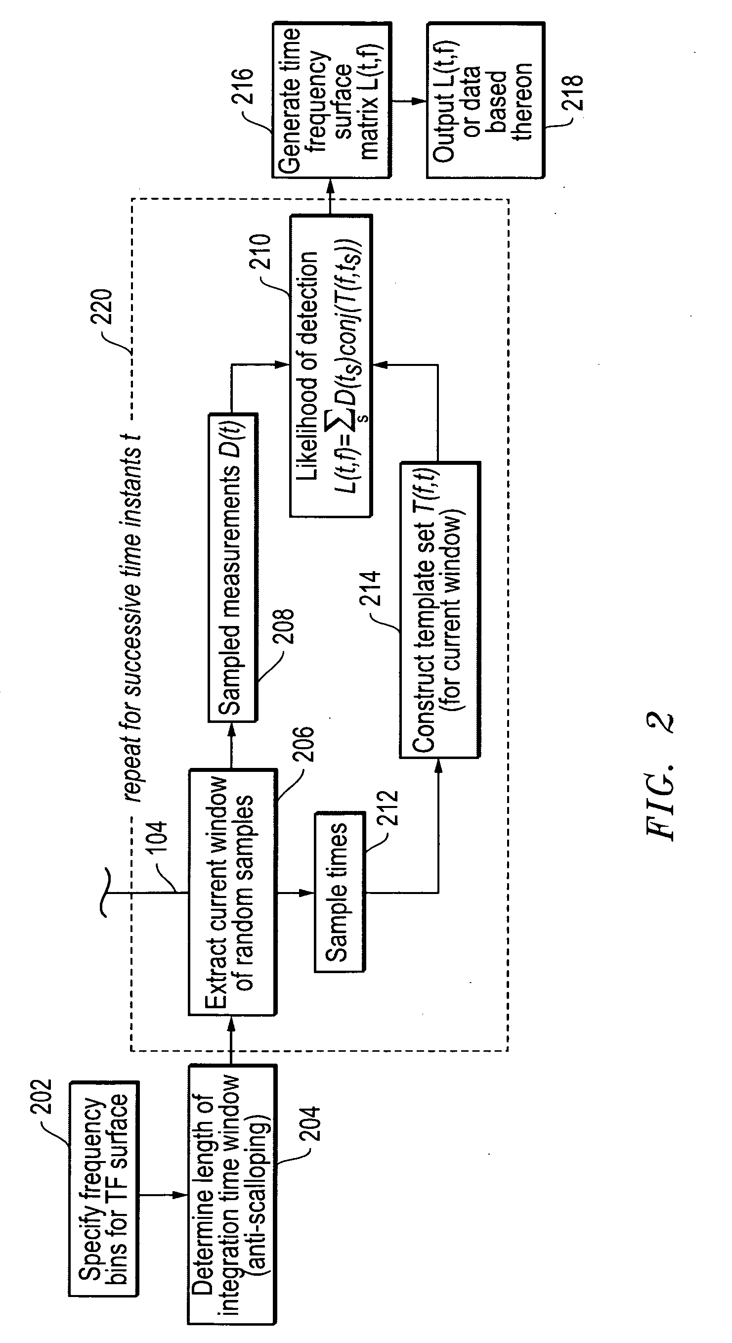
[0055]A randomly-subsampled version of the simulated input signal data of Example 1 was extracted for streaming time-frequency analysis by random decimation, i.e., by randomly selecting 10% of the original samples of the input signal data. As in FIG. 6, 100 frequency bins were selected, with equal spacing between 0 and 50 MHz. A time integration window of 50 samples was chosen. FIG. 7A depicts the TF surface generated using the methodology described and illustrated herein in relation to FIG. 2. FIG. 7B is a time average of the TF surface of FIG. 7A. The first CW tone source is preserved in FIGS. 7A and 7B because it matches the template spacing in a manner as illustrated and described in relation to FIG. 4. The second CW tone source is lost due to frequency scalloping in FIGS. 7A and 7B because it lies between templates in a manner as illustrated and described in relation to FIG. 3. The third signal (the chirpe...
example 3
Randomly Sub-Sampled Data Using Streaming Time-Frequency (TF) Methodology with Reduced Integration Times to Mitigate Frequency Scalloping Loss
[0056]A randomly-subsampled version of the simulated input signal data of Example 1 was again extracted for streaming time-frequency analysis by random decimation, i.e., by randomly selecting 10% of the original samples of the input signal data. For the analysis of this example, 100 frequency bins were once again selected, with equal spacing between 0 and 50 MHz. A reduced integration length of 11 samples was chosen to coarsen frequency-domain and reduce frequency scalloping loss. This reduced length was determined based on a relationship between integration time τ and frequency-bin separation Δf for 50% scalloping loss. This was derived previously above:
τ=0.604Δf
[0057]For 100 frequency bins distributed between 0 and 50 MHz, Δf is 0.5 MHz, resulting in a value for τ of 1.2 μs. The original sample rate of 100 MHz was randomly decimated to 10% o...
PUM
 Abstract
Description
Claims
Application Information
 - R&D
- Intellectual Property
- Life Sciences
- Materials
- Tech Scout
- Unparalleled Data Quality
- Higher Quality Content
- 60% Fewer Hallucinations
Browse by: Latest US Patents, China's latest patents, Technical Efficacy Thesaurus, Application Domain, Technology Topic, Popular Technical Reports.
© 2025 PatSnap. All rights reserved.Legal|Privacy policy|Modern Slavery Act Transparency Statement|Sitemap|About US| Contact US: help@patsnap.com


