Coded filter
a filter and coded technology, applied in surveying and navigation, wave based measurement systems, instruments, etc., can solve problems such as errors in positional calculations in navigation systems, complex environments, and challenge existing kalman filter based systems
- Summary
- Abstract
- Description
- Claims
- Application Information
AI Technical Summary
Problems solved by technology
Method used
Image
Examples
example 1
[0052]In this example, a coded filter is applied to a Kalman filter state estimator. The coded filter modifies the dynamic state estimation algorithm used by the Kalman filter by estimating the vectors etp (non-Gaussian process noise) and ets (non-Gaussian sensor noise) at each time step, and using these estimates to correct the Kalman filter update and propagation steps, as discussed further below. The following formulation is accurate when the error vectors are compressible at each time step. Examples include sensor measurements where at any point in time only a small fraction of the sensors experience non-Gaussian noise, and propagation disturbances that affect only a small subset of the state variables.
[0053]According to one embodiment, for this example, the linear dynamic and measurement model of Equation (1) above can be rewritten in matrix form as follows:
[0yt]=[-Ft-1I0Ht]·[xt-1xt]+[-vt-1wt]+[-et-1pets](17)
As in a conventional Kalman filter, the assumption can be made that xt...
example 2
[0057]The Kalman filter assumes linear propagation and measurements. The above-discussed process for the Kalman filter example (Example 1) may be extended to non-linear propagation and measurement functions by applying conventional linearization techniques used in the derivation of the extended Kalman filter. As discussed above, the evolution of the state of a non-linear dynamic system over time is governed by a non-linear function gt and can be modeled according to Equation (2) above. Equation (2) may be approximated by using a first order Taylor series around the current estimate of the mean ût−1:
xt=gt(ût−1)+Gt−1(xt−1−ût−1)+νt−1+et−1p+errt−1g (23)
In Equation (23) the matrix Gt−1 is the Jacobian of gt−1 at ût−1 and the error vector errt−1g, is the difference between the approximation (using the first order Taylor series) and the actual value of the non-linear function (i.e., the linearization error). As discussed above, a non-linear observation of this process at time t is governe...
example 3
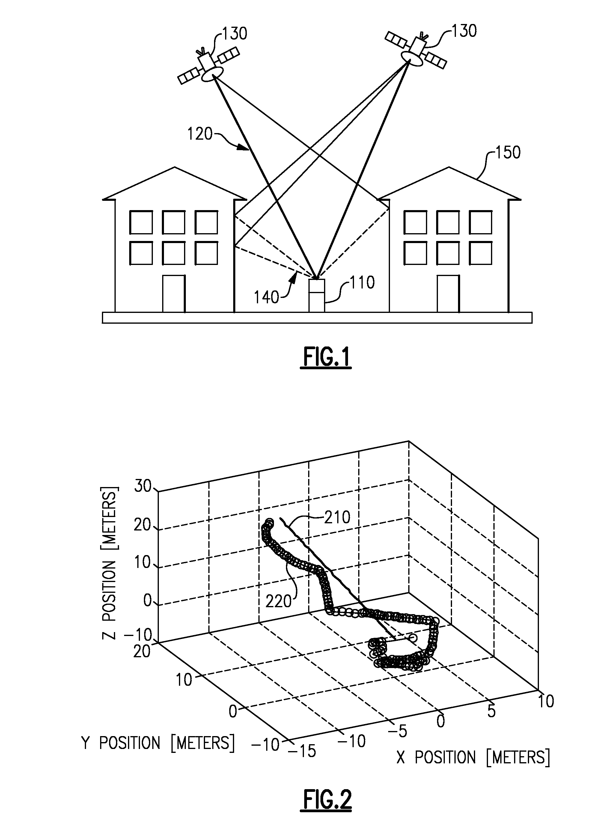
[0060]The Kalman filter (Example 1) and extended Kalman filter (Example 2) coded filtering processes discussed above may apply in cases where the non-Gaussian errors are compressible at each time step. However, there exist cases where the non-Gaussian errors are compressible across time, but necessarily at each point in time. Some examples include sensor measurements where a significant fraction of sensors experience non-Gaussian noise that is structured over time. For example, in the navigation context, this situation may exist where a majority of the GPS channels are corrupted by multipath, but the environmental geometry causing the multipath reflections does not vary too rapidly.
[0061]Therefore, according to one embodiment, a batch formulation of the estimation problem for the linear dynamic system defined by Equations (1) and (4) is used. The batch formulation groups together measurements over a predetermined time frame to create a collection of measurements that can be analyzed...
PUM
 Abstract
Description
Claims
Application Information
 - R&D
- Intellectual Property
- Life Sciences
- Materials
- Tech Scout
- Unparalleled Data Quality
- Higher Quality Content
- 60% Fewer Hallucinations
Browse by: Latest US Patents, China's latest patents, Technical Efficacy Thesaurus, Application Domain, Technology Topic, Popular Technical Reports.
© 2025 PatSnap. All rights reserved.Legal|Privacy policy|Modern Slavery Act Transparency Statement|Sitemap|About US| Contact US: help@patsnap.com


